
Stable, what a beautiful word! With OPAMP in a “stable” circuit, we don not need to worry about oscillation and so many other problems. However, under many circumstances, circuits we design are not stable, which we call “conditionally stable”. In this article, we’ll find out what stability is and how it is related to RF amplification design.
Power gain in a two-port amplifier
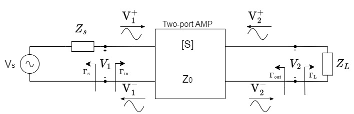
Figure 1 shows a diagram of a two-port amplifier
Before doing mathematical calculations, we shall define three different two-port power gains as follows:


![\left[ S \right]](https://s0.wp.com/latex.php?latex=%5Cleft%5B+S+%5Cright%5D&bg=ffffff&fg=000&s=0&c=20201002)


When load side and source side are both conjugate matched, we have

Gain Calculation
The reflection coefficient seen looking toward the load is

while the reflection coefficient looking toward the source is

Generally, both sides of the amplifier are not well matched and we can derive


then we can derive


From voltage division

and by the definition of reflection coeficient

If we solve


and if peak values are assumed for all voltages, the average power delivered to the network is

As for the power delivered to the load

so power gain is

If we are calculating available power gain, there should be conjugate matching on the source side, which means

and when

Similarly, when there is conjugate matching on the load side,

However,


and


Now both

So, the available and transducer power gain is

When both source side and load side are matched(


When


and the unilateral transducer power gain can be given in a format with symmetrical beauty and balance.

Single-Stage Amplifier
A single-stage microwave amplifier can be modeled by the circuit in figure 2.

In figure 2,a matching network is added on both source and load side to transform the input and output impedance

and the overall transducer gain is

Furthermore, we assume the circuit is unilateral(

The alternative results can also be derived from small signal model of this circuit.
Stability Circle
In the circuit of figure 2, oscillation may occur if either the input or the output port impedance has a negative real part, which will imply that


- Unconditional stability The network is unconditionally stable when
- Conditional stability The network is conditionally stable when


Besides, the stability condition of an amplifier circuit is usually frequency dependent. It is therefore possible for an amplifier to be stable at its design frequency but unstable at other frequencies.
When a circuit is unconditionally stable, we have

If the circuit is unilateral, the conditons above can be reduced to

Otherwise, the inequalities define a range of values for


We can derive the equation for the output stability circle as follows.

Now we define


Then the output stability circle can be written as

and we square both sides and simplify

And we add


In the complex


Similarly, the input stability circle can be defined as:

Now we know how to draw a stability circle and we know on the one side of the circle, the circuit is stable while on the other side, it’s not. Here comes the question: which side is stable and which side is unstable?
Consider the output stability circle plotted as figure 3 shows in the complex


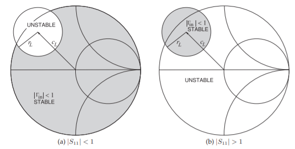
Now we go back to the origin equation


This result is shown in figure 3.
Test for Unconditional Stability
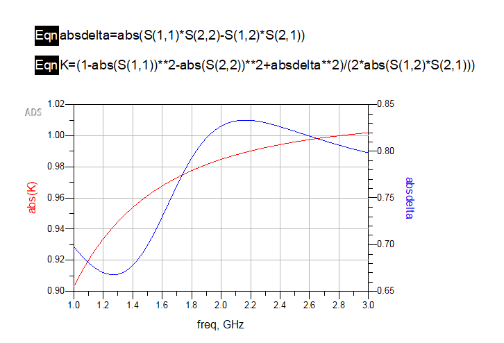
The stability circle is a way to determine where the amplifier will will be unstable in the complex reflection coefficient plane. However, there is a simple way to determine unconditional stability, which is K-Δ test.

If the two conditions are met simultaneously, then the amplifier is unconditionally stable.
One Example in ADS
Let’s see an example in ADS which is a single -stage amplifier.
In 07_SP_Matching of this project, we can add two equtions to test its stability as shown in figure 4. We can see the amplifier we design is conditional stable at 2 GHz. We can also use StabFact component to derive K.
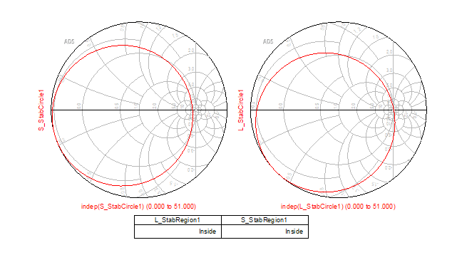
Then let’s see what the stability circle looks like at 2GHz. We can use S_StabCircle and L_StabCircle to draw the circle and use S_StabRegion and L_StabRegion to determine the stable region.
Reference
Microwave Engineering by David M. Pozar

Leave a comment